Working with Raster
Introductions
In this page, we demonstrate how to extract values from maps using R. Often we have maps showing values for each pixels, for example, ITN access and usage map with 5km x 5km resolutions or Population counts with 1km x 1km resolutions. To convert these maps to useful estimates for our model, we need to extract the values underlying each pixel in the map, within the geographical area of interest. For example, if the map covers the entire Sub-Saharan Africa, and all we need is values from Burkina Faso, we will need to only extract the pixels within the country’s boundary. Then we would need to aggregate the values of the pixels, to obtain some form of country-wide estimate. Similar analogy is applicable to region, district and province.
We use the sp and raster packages in R to achieve this. For the first example, we will walk through extracting ITN usage estimate for a Burkina Faso district of Kampti.
Example 1: ITN usage of Kampti District
To achieve this, it is important to look at the “ingredients” needed:
- Shape file for Burkina Faso and its district (You need to unzip this)
- 2016 ITN usage map (note that this is originally covering the entire of SSA, but is cropped to reduce filesize)
- 2016 estimated population distrbution map of Burkina Faso
Shape file serves as a “cookie cutter” such that we can ensure to extract values within the boundary of a district or area of interest. We will discuss about the use of population distribution map later.
Here are the code walkthrough. First we import the libraries, and load the input using raster() and shapefile() functions.
library(sp)
## Warning: package 'sp' was built under R version 4.1.3
library(raster)
## Warning: package 'raster' was built under R version 4.1.3
shp <- shapefile("data/burkina_70DS.shp")
shp
## class       : SpatialPolygonsDataFrame
## features    : 70
## extent      : 224822.8, 1088963, 1040345, 1669090  (xmin, xmax, ymin, ymax)
## crs         : +proj=utm +zone=30 +datum=WGS84 +units=m +no_defs
## variables   : 11
## names       : OBJECTID,  NOMDEP, SinistreIn, Innonde, NOMPROVINC,         NOMREGION, CommuneCib, CoomuneRis,    Shape_Leng,    Shape_Area, DS
## min values  :        7, BANFORA,          0,       0,       BALE, BOUCLE DU MOUHOUN,          0,          0,  22326.136677, 28397716.1216,  0
## max values  :      107,  ZORGHO,       3179,       1, ZOUNDWEOGO,         SUD-OUEST,          1,          1, 656058.771223, 14845528347.3, 69
itn_raster <- raster("data/ITN2016.tif")
itn_raster
## class      : RasterLayer
## dimensions : 156, 216, 33696  (nrow, ncol, ncell)
## resolution : 0.04166665, 0.04166665  (x, y)
## extent     : -6.00007, 2.999927, 8.999972, 15.49997  (xmin, xmax, ymin, ymax)
## crs        : +proj=longlat +datum=WGS84 +no_defs
## source     : ITN2016.tif
## names      : ITN2016
## values     : 0.09760008, 0.8092381  (min, max)
pop_raster <- raster("data/bfa_ppp_2016_1km_Aggregated_UNadj.tif")
pop_raster
## class      : RasterLayer
## dimensions : 682, 951, 648582  (nrow, ncol, ncell)
## resolution : 0.008333333, 0.008333333  (x, y)
## extent     : -5.517917, 2.407083, 9.407917, 15.09125  (xmin, xmax, ymin, ymax)
## crs        : +proj=longlat +datum=WGS84 +no_defs
## source     : bfa_ppp_2016_1km_Aggregated_UNadj.tif
## names      : bfa_ppp_2016_1km_Aggregated_UNadj
## values     : 0.2217675, 6855.859  (min, max)
The summaries for each of the object suggests that shp has a different CRS (Coordinate Reference System) than others. The CRS of all objects must align for our work here, and it’s easier to convert CRS in shp to that of other raster objects.
shp <- spTransform(shp, crs(itn_raster))
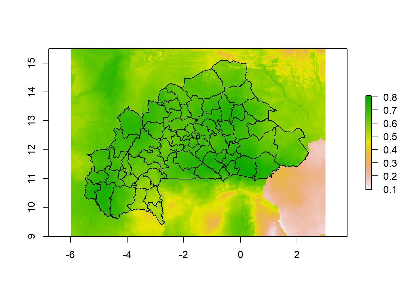
Now we can plot and see the raster and shapes. Here’s ITN raster.
plot(itn_raster)
plot(shp, add=T)
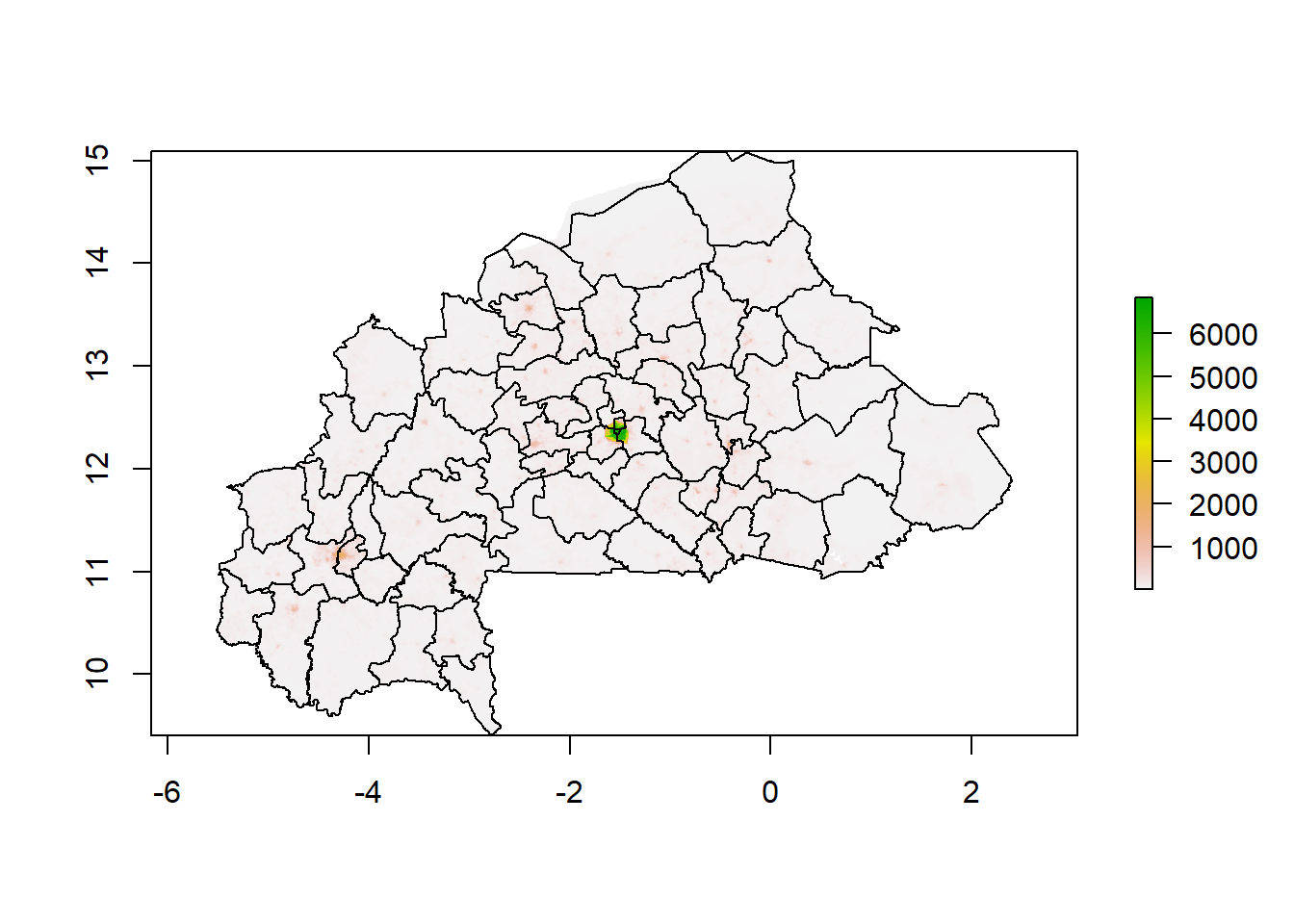
And here’s population raster. There are a little misalignment in the north for this raster, but for our purpose, this problem is not too big.
plot(pop_raster)
plot(shp, add=T)
Naïve Extraction
The most naïve way of extracting values for each district here is to directly use the extract() function. When supplied with a set of polygons (shapes), the function pull the values underlying all the pixels within the shapes, and aggregate them, say by taking means. The function can be supplied by a set of points too.
df <- shp@data # Pull data out of shapefiles (District names etc.)

# Extract and aggregate using mean function
df$itn_cov <- extract(itn_raster, shp, fun=mean)

# Look at values for Bittou district
df[df$NOMDEP=='BITTOU', c('NOMDEP', 'NOMREGION', 'itn_cov')]
##    NOMDEP  NOMREGION   itn_cov
## 53 BITTOU CENTRE-EST 0.7512201
Population-weighted extraction
Sometimes averaging each pixel without weights doesn’t feel quite “right”: Pixels inside uninhabited forests aren’t the same as pixels inside a crowded town when we care about ITN coverage. Therefore, we may elect to use population map to weight the pixels and obtain a population-weighted estimate for each district.
# First try to stack the ITN and Population map
## To do so, need to ensure two maps cover same area
## Crop ITN raster according to Population raster
itn_raster_cr <- crop(itn_raster, pop_raster)
## Lower resolution of Population raster to the level of ITN raster
pop_raster_res <- resample(pop_raster, itn_raster_cr, )

## Stacking the raster
itn_pop_stack <- stack(itn_raster_cr, pop_raster_res)

# Extract the raster stack according to the shapes, no aggregation
out <- extract(itn_pop_stack, shp)

# Define functions to calculate weighted average from output matrix
weighted_avg <- function (x, w) sum(x * w) / sum(w)
estim_from_matrix <- function (mat) {
  mat <- na.omit(mat)
  return(weighted_avg(mat[,1], mat[,2]))
}
Without specifying the aggregating function for extract(), the function pull every single pixel out of the raster stack. Result is a list of matrices, first column is ITN coverage, second column is population count. So we define a function estim_from_matrix() that would calculate weighted average of first column according to second column. sapply() applies the function to each element (matrix) of the list, and combine the output nicely into a vector.
df2 <- shp@data
df2$itn_cov <- sapply(out, estim_from_matrix)

df2[df2$NOMDEP=='BITTOU', c('NOMDEP', 'NOMREGION', 'itn_cov')]
##    NOMDEP  NOMREGION   itn_cov
## 53 BITTOU CENTRE-EST 0.7475682
The ITN coverage estimates from population-weighted method is almost the same as the naive method. This is potentially due to the ITN estimates within the district being relatively homogeneous.